Much of theoretical statistics involves assumptions that rarely apply to real data, and most real data involve multiple complexities in combinations that may not have been studied in detail. For example, there is a substantial literature on what to do about missing data, on how to adjust for temporal auto-correlations (time-series), on how to adjust for hierarchical data structures (multi-level models), and on how to deal with variables having too many zeros. However, I would bet that not a single methodological study has examined how to deal with all four of these challenges simultaneously or considered how they might interact with each other. As a result, the theoretical and methodological literature in statistics is generally not able to furnish us with clear answers to the thousands of such combinations and challenges that confront us daily. The approach outlined here is largely a response to the need to deal with complex data in the absence of clear methodological guidance for specific cases.
Hypothesis testing has a scientific sense and a statistical sense, and we reject both under most circumstances. In a scientific sense, a hypothesis testing framework is too black and white and often prevents us from realizing when the data are telling us we were asking the wrong question. In a statistical sense, the origins are partly due to a historical inability to calculate precise p-values easily. With computers, this is no longer the case. Statistics is about estimating uncertainty in a probabilistic world; trying to take this uncertainty and chop it into “true” and “false” based on an arbitrary p-value threshold is antithetical to basic principles of probability.
Many statistics texts use arbitrary rules and decision trees (e.g., use non-parametric statistics for n < 30). There is generally a good reason to apply such rules in most cases, but there are also many exceptions (e.g., some non-parametric tests may cause an unjustified loss of power for n < 30 when the distribution is known to be normal based on prior knowledge, and non-parametric tests also impose suppositions on the distribution that may not be justified). Blindly applying such rules guarantees that the wrong decision will be made in a substantial minority of situations. The only acceptable solution is to understand where the rules come from and to use careful judgment on a case-by-case basis.
Often, the variable we wish to study cannot be measured directly, and we thus combine many methods to generate variables that better represent the true biological (or sociological, etc.) process we wish to measure. For example, if we want to measure the morphology of babies at birth adjusting for the fact that some are born prematurely, we would need to first run a principal components analysis on various morphological measurements to summarize key aspects of shape. The axes generated by this analysis would then be run through a cubic spline regression on gestational age at birth, and the residuals of this regression would give the variable we desired. Although complex, such approaches are often essential if we wish to measure the true underlying processes of interest rather than the crude proxies that we can measure directly.
This is perhaps the most critical point. Running a statistical analysis involves thousands of arbitrary choices that have the potential to change the results. Do we exclude a height measurement of 203 cm as an outlier? What variable should we use to approximate socio-economic status? Which variables should be log-transformed? What sort of maximum likelihood estimation procedure should we use? Together, the need to make so many choices puts the results of any single analysis in substantial doubt. If you don’t believe this, try the tool here to see how a small number of such choices can completely change the results of an analysis on whether the US economy does better under Republicans or Democrats. There is only one real solution to this problem: run many, many versions of the analysis to see if the results are stable and, if not, which choices affect the results. We typically run tens of thousands of analyses for a single publication. If the results are concordant, we can start to be more certain about the conclusions. If not, we need to understand why there are differences before we can publish.
The replication approach above generates so many results that it is often difficult to sort through them manually. We thus often run analyses on the effects of our alternative analytical approaches on the results. For example, if we have five factors we can vary for a regression analysis with, respectively, 3, 4, 2, 2, and 10 options, we can run 3 x 4 x 2 x 2 x 10=480 analyses to cover all combinations. Then we can put the 480 regression coefficients generated into a meta-regression where we analyze the effects of each of the options for each of the factors on the results. Such approaches are not always needed, but they can provide a rigorous way to evaluate the stability of results and the factors that can influence them.
Particularly for continuous variables, one of the most basic and yet most difficult aspects of statistics is to consider the distribution. Is a variable normally distributed? Is what appears to be a normal distribution actually hiding a mixture distribution based on an important covariable? What does our understanding of the biology tell us about the distributions of the variables, how to transform them, how to treat outliers, etc.? Most discussion of distributions in applied statistics is simple: try to get your variables normal (with, say, a log-transformation). Most discussion of distributions in theoretical statistics is precise: exploring subtle differences among theoretical distributions that might not be distinguishable empirically in most data sets. Neither approach is sufficient in most cases. It is rarely possible to invest too much time thinking through the distributions of the variables, what this tells us about the biology, and how to treat them in subsequent analyses.
Linked to the previous point, one of the biggest errors in many scientific articles is to treat the measured variable as the phenomenon of interest. In most cases, this is not justified: what we can measure is a poor proxy for the true process (biological, sociological, etc.). Consider the figure below, which represents four different ways the clinical threshold for diabetes diagnosis (126 mg/dl) might represent a true underlying process. Most people suppose that, because we say that a person has diabetes if her blood sugar is higher than 126 mg/dl, then the top left model is the correct one. Confronted with these figures, however, most would agree that the top right or bottom left figure is closer to the true model. Even if we continue to measure diabetes as a dichotomous variable, having considered the underlying process may lead us to run different statistical models and ask different scientific questions. (In fact, different statistical models are ALWAYS different scientific questions…) In the best case scenario, failure to consider underlying processes leads to researchers ignoring measurement error. More commonly, it leads to the asking of nonsensical questions or the generation of spurious results.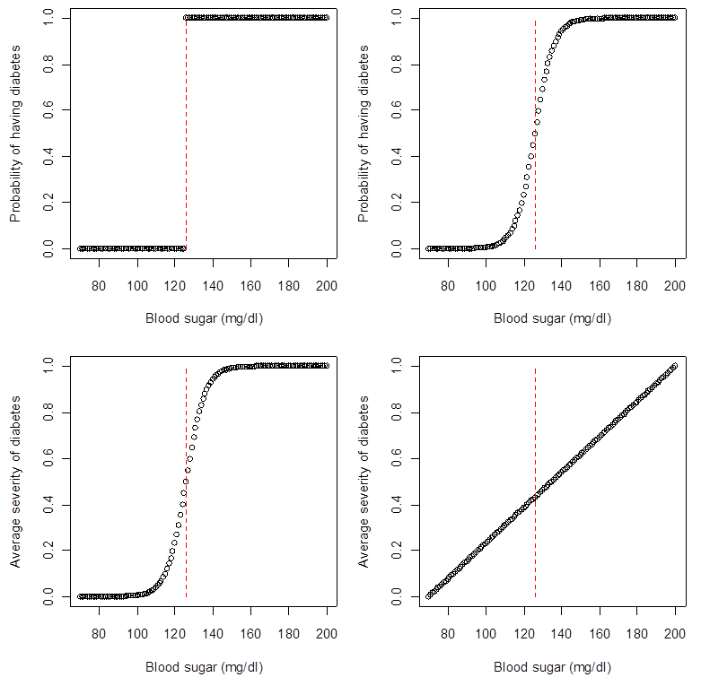
Our brains are wired to simplify things, and one important way we do that is to notice uncertainty temporarily and then ignore it. We read a scientific article, read and acknowledge its limitations sections, but when we cite or apply the article, we usually assume it is simply true (or simply false). We do the same thing in statistical analysis, ignoring the uncertainty from previous levels of analysis and thus placing too much faith in the final analysis (and final estimate of uncertainty). There is no simple recipe to avoid this error other than to be conscious of the risk and to try to adjust for it appropriately.
The approaches outlined above – particularly replication of results in multiple analyses and contexts – are not a panacea. In particular, there is a risk that many analyses contain the same bias. If it is important to control for socio-economic status (SES) in an analysis and the SES measure is too imprecise, many different analyses may show the same spurious effect because they all share the same bias.
We all have personal biases and results that we expect or would like to observe. In some cases, these may be professional or financial biases such as the need to publish in a high-impact journal for promotion or a pharmaceutical company trying to gain regulatory approval. Many of the rules surrounding statistical practice are designed to avoid these biases – some examples include formulation of a priori hypotheses and adjustment for multiple testing. However, these rules are far from sufficient, as can be seen from the much higher probability that a study will support a pharmaceutical product if it is financed by a company with a financial stake. The rules may not be useless, but bias is still a major problem, and the rules have a substantial cost: they make us rigid and unable to follow the evidence wherever it takes us. For example, a medication that was supposed to reduce breast cancer mortality may fail to achieve its desired effect, but may substantially improve quality of life. We should not discard the finding on quality of life simply because we did not predict it, but we should be cautious about over-interpreting it if the effect is weak or marginal.
The best solution to the aforementioned problem of bias is not a series of rules, but rather an honest attempt by researchers to combat these biases and prove themselves wrong. Obviously, not all researchers will do this well, and some will not even try. It is thus also up to reviewers and editors to demand a more nuanced and self-critical approach to research in the articles we review.
Generating thousands of results per article is a challenge for writing up clear, concise articles. We take the following approach: (1) Conduct enough analyses that we are confident about the take-home message (even if the message is a nuanced or subtle one). (2) Write the article around this message. (3) Include sufficient detail in the Methods and Supplementary Information to show readers that we have tried many, many variants on the analysis. (4) For simplicity, omit descriptions of analyses that are not central to understanding the take-home message, even if they helped us get there. (5) Write articles so as to encourage other researchers to copy this approach.